Build the Laboratory, Not the Legend

This is not betting advice. It is a description of research infrastructure built to separate real signal from well-formatted randomness.

After the first version, we had a lot of code, a lot of reports, and enough stage names to make a modest space agency feel underbranded.

What we did not have was a foundation we could trust without adding:

“Well, the script completed successfully.”

The rebuild did not begin with another algorithm. It began with a more uncomfortable question:

Do the data, labels, and timestamps actually mean what we think they mean?

It is a boring question.

That is precisely why it belongs near the entrance of every laboratory.

First, remove the architectural nesting dolls

Long projects develop a dangerous habit: every new solution is placed carefully on top of the old one.

The old script almost works? Add a wrapper.

The wrapper lacks one function? Patch it at runtime.

The new stage depends on the previous stage? Import the whole thing and call its main().

A few months later, understanding one command requires opening three scripts, two configuration files, and a small portal to the universe where final_v17_really_final.py is considered a normal filename.

Our first rebuilt preparator did exactly this. It imported the old a0_prepare_dataset.py, replaced several functions at runtime, and presented the result as the new version.

There are legitimate reasons to do that during a migration. It keeps the diff small and lets a prototype reuse tested code.

As a final architecture, it was wrong for this project.

The owner should not need to guess which implementation actually ran. A daily command should not secretly summon an earlier stage, alter its memory, and return everything before anyone notices.

We stopped and wrote down one rule:

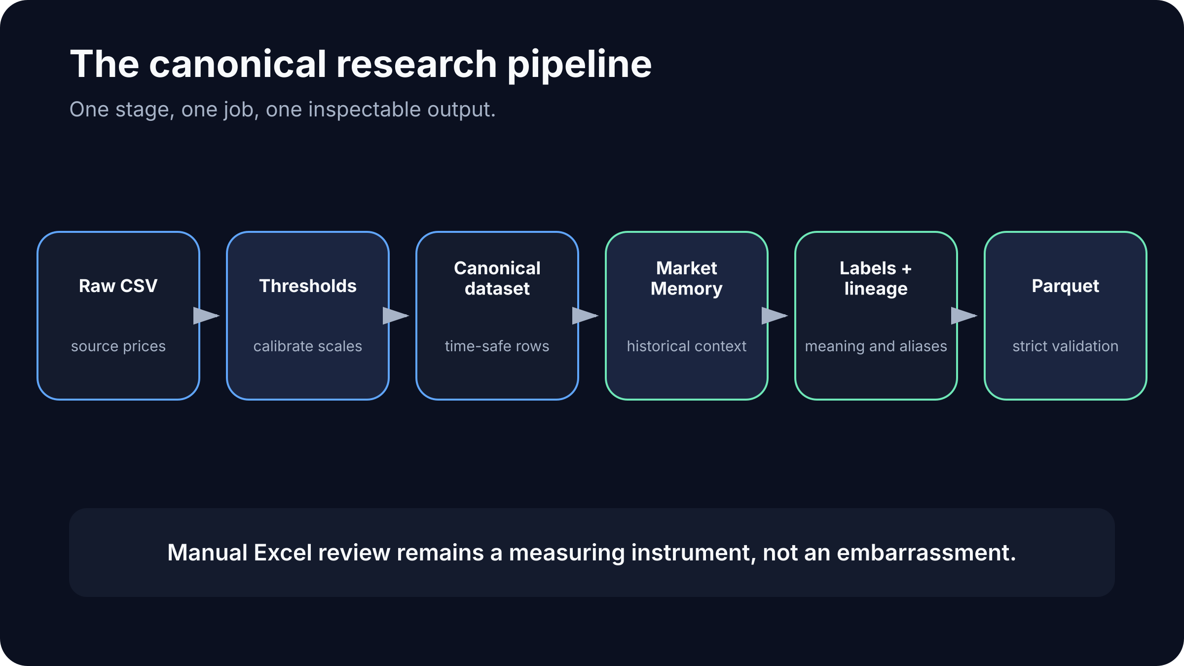
One stage, one job, one inspectable output.

The canonical path became:

mlb_raw.csv
→ a0_calibrate_trend_thresholds_mlb.py
→ mlb_trend_thresholds.json
→ a0_prepare_dataset.py
→ mlb.csv
→ historical features
→ labels and lineage
→ strict Parquet conversion

No hidden import from a later stage. No monkey-patching. No script that needs another script to pretend it is itself.

The error hidden inside two valid formulas

One of the most important discoveries was not inside a prediction model. It was in the movement contract.

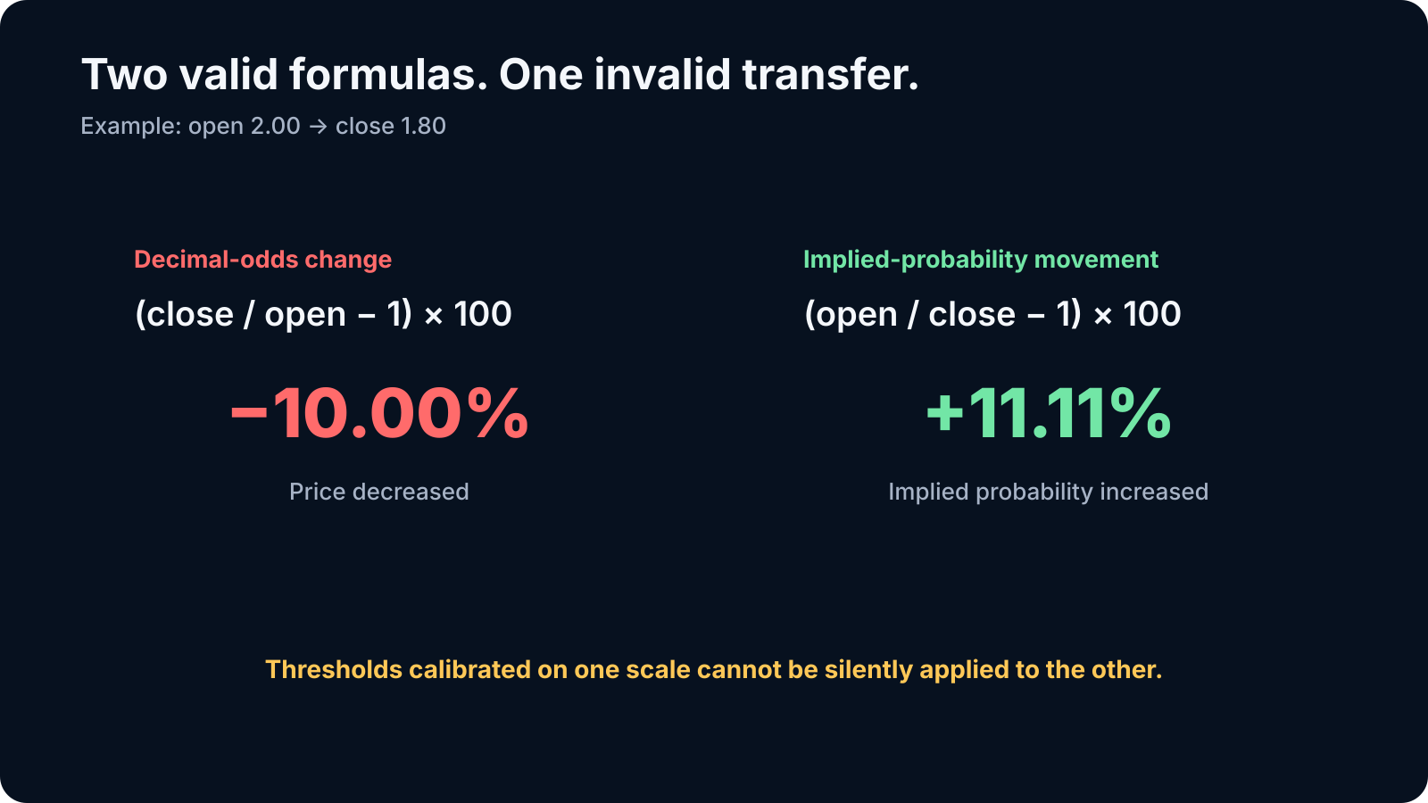
The old pipeline calculated movement with one formula while applying thresholds calibrated on another.

The current calculation was:

(close / open - 1) × 100

The stored p75/p90/p95 thresholds had been calibrated on relative implied-probability movement:

(open / close - 1) × 100

Both formulas are legitimate.

The mistake was their marriage.

Take a simple example:

open  = 2.00
close = 1.80

The decimal price changed by:

(1.80 / 2.00 - 1) × 100 = −10.00%

The relative implied probability changed by:

(2.00 / 1.80 - 1) × 100 = +11.11%

The sign changes. The magnitude changes too.

For small moves, the two scales look almost like mirror images, which allows the mistake to remain respectable for a surprisingly long time. The table still opens. The chart still has axes. Nobody receives an emergency alert saying, “Congratulations, Celsius thresholds are now interpreting Fahrenheit.”

We chose one contract:

MOV = (open / close - 1) × 100

A positive value means implied probability increased and the decimal price shortened. A negative value means the opposite.

Human-readable suffixes continued describing the decimal odd itself:

MNS → closing odd is lower than opening odd
PLS → closing odd is higher than opening odd
FLT → movement is effectively flat

So a positive MOV can end in MNS. That is not a contradiction. The formula describes implied-probability movement; the suffix describes the visible decimal price.

The math must be precise. The label must remain readable. They are allowed to look at the same event from opposite sides of the glass.

Think in matches, not folders

The old system often thought in daily batches: yesterday, today, a date folder, a slate.

Sports do not respect our folder structure.

A match can begin before midnight and finish after it. Another can start shortly afterward. If the entire “previous day” is admitted into history, the laboratory may use a result that was not known at the target time.

We did not have exact settlement timestamps. So we defined a conservative, explicit proxy:

historical Event_Start_UTC + 12 hours
<
target Event_Start_UTC

Only then is the historical result considered available.

It is not a claim about perfect physical truth. It is a testable information contract attached to each match rather than to a calendar folder.

Why 12 hours? Most games finish much sooner. The buffer covers late starts, extra innings, delays, settlement lag, and a healthy amount of distrust. Twenty-four hours would be safer but would discard much of the previous night. We chose 12 and retained 24 as a sensitivity option.

The important part is not that 12 is sacred.

The important part is that the boundary is explicit.

A completed match counts even if the season is still alive

One intermediate implementation excluded the current season from common threshold calibration because the season had not formally ended.

It looked tidy. It did not match our actual research unit.

We analyze completed matches, not completed calendar folders.

If one thousand events from the current season have finished, they are one thousand real observations. They should not be exiled because future fixtures still exist.

The revised principle was simple:

A completed match participates. An incomplete match does not.

Seasons remain useful for stability checks and separate partitions. They do not decide whether an observation has the right to exist.

Individual and global are different rulers

The same percentage move does not mean the same thing at every bookmaker.

A 6% move may be extreme for a quiet source and routine for a volatile one.

So we created parallel scales:

TRNDI_* → individual thresholds for each bookmaker
TRNDG_* → global pooled thresholds across real bookmakers
TRNDA_* → separate aggregate layer for AVG / MIN / MAX

TRNDI had to remain genuinely individual.

If a source lacked its own opening pair or enough history, the value stayed empty. We did not borrow AVG role, apply the source's threshold, and call the result an individual label.

That hybrid would look like this:

BWIN movement
+ AVG role
+ BWIN threshold
= allegedly pure BWIN state

It is a composite wearing an individual trench coat.

Globa refused it entry.

Choosing a useful movement language

The first movement grid used:

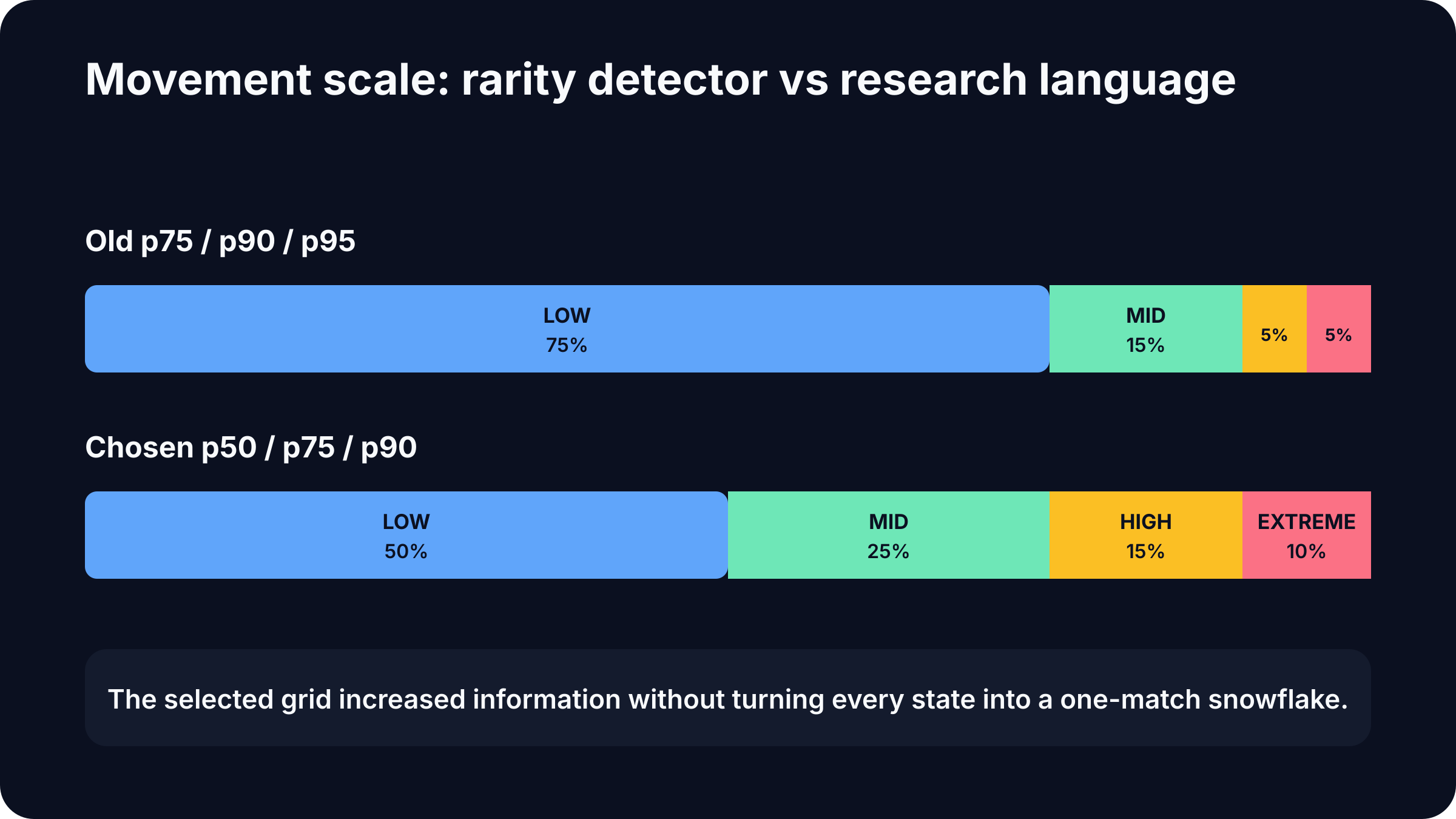
p75 / p90 / p95

It produced approximately:

LOW       75%
MID       15%
HIGH       5%
EXTREME    5%

That is sensible for a rarity detector. It was less useful as a research language because LOW became a warehouse containing nearly everything.

We compared three schemes without using outcomes or ROI:

A: p75 / p90 / p95
B: p50 / p75 / p90
C: p50 / p65 / p80 / p90

The comparison focused on representation quality:

• how evenly the states were used;
• exact-state support;
• micro-sample frequency;
• seasonal stability;
• how quickly the space fragmented when conditions were combined.

Scheme B provided the best balance:

LOW       < p50       ≈ 50%
MID       p50–p75     ≈ 25%
HIGH      p75–p90     ≈ 15%
EXTREME   ≥ p90       ≈ 10%

Median support for a bookmaker trend pair increased from about 17 to 28 matches, while the share of states with N < 25 fell. The five-bucket grid added detail but fragmented the space faster.

That ordering mattered. A label system should be chosen before it sees which outcomes make it look clever.

Equal odds are not missing data

Previously, a null could mean several different things:

• no price;
• one side missing;
• invalid data;
• exactly equal opening odds.

Those are not the same state.

An equal line is real market information. It says the source did not identify a favorite at that precision.

We added explicit roles:

FAV_1
FAV_2
EQUAL
NO_DATA

At 1.86 / 1.86, we do not invent a favorite. We do not borrow AVG so that the table looks more complete. Equality and absence belong in different drawers.

A laboratory should not label both drawers “something happened, probably.”

The canonical dataset

After the hardening pass, the MLB research object contained:

9,492 matches
1,275 columns
17 active Market Memory sources
unique non-null Match_ID

Major families included:

TRNDI_*          54
TRNDG_*          54
TRNDA_*           6
ODDSROLE_*       60
ODDSLVL_*       120
MOV_*            60
MM_*            516
feature labels  245

The strict CSV-to-Parquet converter validated 891 numeric columns. No valid number became a new null.

That sounds like a technical footnote until you remember that an earlier conversion path could attempt to cast string fields such as TRNDG_* states or MM_*_SIDE into Float32 and quietly erase them.

Sometimes the most valuable feature of a research platform is preventing the table from disappearing with a calm expression.

What Market Memory measured

Market Memory asked a narrow question:

How did earlier matches finish when this source showed a similar opening market state?

A memory key included:

history partition
+ canonical favorite side
+ source's favorite opening odd rounded to two decimals

For each source, the system calculated:

• historical sample size;
• favorite and underdog wins;
• historical fair percentage;
• fair odd implied by that percentage;
• current market probability;
• difference between memory and market;
• consensus and dispersion;
• pairwise source differences;
• strict and overall head-to-head context.

The result was *516 `MM_` columns**.

But 516 columns are not 516 independent ideas.

For example:

FAIR_PCT = WINS / TOTAL
FAIR_ODD = 100 / FAIR_PCT
VALUE_PCT = −EDGE_PCT
MARKET_PCT = 100 / ODD

These are different views of related information.

A rich dataset is useful. A rich dataset that forgets family relationships becomes an algorithm factory with a costume department.

245 labels, 109 rule-enabled fields, 74 independent groups

Numeric fields are useful for models. Humans often understand discrete labels more quickly.

We added labels for:

H2HPCT_*
H2HSUP_*
MMPCT_*
MMEDGE_*
MMSUP_*
MMCONS*
MMDIFF_*

There were 245 new label columns.

Only 109 were technically allowed in later rule analysis. After lineage was counted, those represented 74 independent rule-enabled groups.

Why the reduction?

Because:

MMPCT_B365_FAV
MMPCT_B365_DOG

are complementary views of one probability.

And:

MMEDGE_B365_FAV
MM_B365_FAV_VALUE_PCT

are the same quantity with opposite signs.

The 136 pairwise MMDIFF fields remained available for audit and manual inspection, but the automatic rule generator was not allowed to multiply them into millions of supposedly independent discoveries.

That is the difference between having many measurements and pretending to have many witnesses.

CSV first, Parquet second

We deliberately kept a human-review stage:

mlb.csv
→ mlb_features.csv
→ mlb_features_labeled.csv
→ manual Excel review
→ mlb_dataset.parquet

Parquet is faster. Excel lets the owner point at one row and ask:

Why does this say MOV = 0.21 when the visible values look like 1.78 → 1.78?

That question exposed global two-decimal display rounding that hid internal precision. We fixed the presentation, regenerated the data, and checked again.

Manual inspection is not an embarrassing legacy inside a sophisticated laboratory.

It is a measuring instrument.

The point is not to replace human inspection with code. The point is to make code produce objects that a human can inspect without prayer.

What we gained before testing a single new candidate

At the end of the rebuild, we still had no production candidate.

We had something more basic and more valuable: an object capable of answering strict questions.

• Where did this feature come from?
• Was it available before the target match?
• Which historical sample produced it?
• How large was that sample?
• Which fields are aliases?
• Which source has real coverage?
• Which exact Match_ID values sit behind the aggregate?
• Did conversion silently destroy anything?

This was no longer a legend about a model.

It was a laboratory.

Part III uses that laboratory for its intended purpose. Market Memory, H2H, consensus, opening states, movement, manual samples, and cross-book spreads are compared with the bookmaker market—not with zero, not with a flattering slice, and not with a graph whose y-axis begins wherever morale requires.

Then one result appears to make money.

Globa reaches for the approval stamp.

AGI asks which price was actually available.