Make the Miracle Show Its Papers

This is not betting advice. Every result below is a historical research test. When the quoted price could not have existed at the time the signal became knowable, the result is treated as a diagnostic—not as a strategy.

Once the rebuilt laboratory was ready, the temptation was obvious. With 1,275 columns and enough states to make the old seven-million-rule search look like a warm-up, we could simply ask the computer to find something profitable.

We did the opposite. Each feature family received one narrow question. No fresh combinatorial sweep, no choosing the best bookmaker after seeing the race, and no moving the goalposts until they formed a decorative arch around one positive row.

The new rule was:

First test whether the mechanism adds information. Only then discuss a candidate.

And every mechanism had to face the market.

The market became the control group

A model that says the favorite has a 60% chance can sound useful.

If the no-vig market already says 63%, the model has not added information. It has created a less accurate retelling of the same forecast.

For probability tests, we used Brier score: squared error for probability forecasts, with confident mistakes punished more heavily than cautious ones. Think weather: being wrong after saying “55% chance of rain” hurts less than being wrong after saying “99%.” Lower is better.

The gate was simple:

An opening-safe feature must improve the opening no-vig probability. A feature known only near close must improve the closing no-vig probability.

Comparing with 50%, the overall home-win rate, or zero ROI was no longer enough. The bookmaker price was not decoration around the experiment. It was the control group.

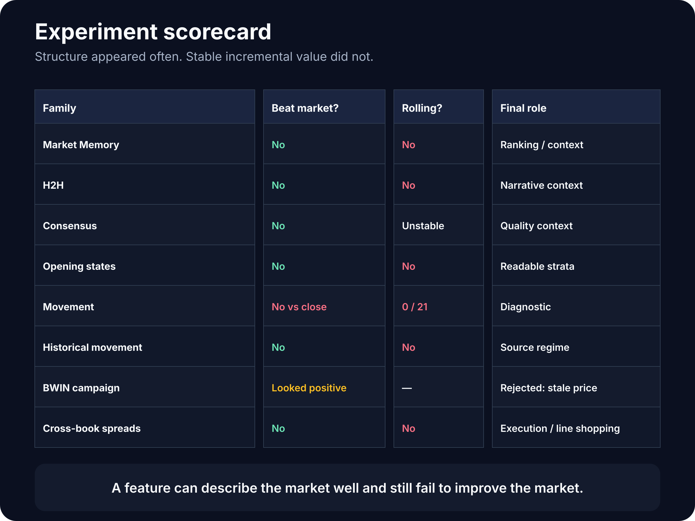
The table is mercifully short. Behind it sit dozens of reports, many rolling folds, and enough coffee for the market to feel like an unannounced relative.

Market Memory: the ranking lived, the probability lied

Market Memory asked how earlier matches had finished when a source showed a similar opening state.

A field such as:

MMPCT_B365_FAV = 65

meant that the canonical favorite had won roughly 65% of earlier matches in that B365 memory state.

The first response test found something real:

• in 12 of 17 favorite-side source lanes, higher MMPCT corresponded to higher future win rates;
• the same was true in 12 of 17 underdog-side lanes;
• the ordering often survived confirmation;
• honest numerical calibration succeeded in 0 of 34 source-side lanes.

In other words:

65 was usually stronger than 55

but:

65 did not mean a reliable 65%

A thermometer can rank warm days above cold days while printing the wrong temperature on every screen.

We then shrank Memory toward the market:

p_final = p_market + λ × n/(n+k) × (p_memory − p_market)

Small samples received less weight; large samples received more. Discovery selected only:

λ = 0.10

Even training said: trust just ten percent of Memory's disagreement with the price.

On frozen confirmation:

Market Brier:       0.243597
Shrinkage Brier:    0.243611

The adjusted Memory estimate was slightly worse. Rolling 3M/1M and 6M/1M checks did not rescue it. In several folds, training selected λ = 0—the model's polite way of saying:

Thank you for the historical context. Please do not touch the probability this month.

Market Memory remained useful for ranking and description. It did not earn the job of primary probability engine.

Globa wrote in the notebook:

“Ordering alive. Probabilities occasionally imaginative. No production access.”

MMEDGE: elegant mechanism, missing gradient

MMEDGE compared the historical fair probability with the current market-implied probability.

The story was attractive:

EDGE < 0 → market knows more
EDGE ≈ 0 → neutral
EDGE > 0 → memory sees value

If the mechanism were broad and real, increasing MMEDGE should produce a reasonably monotonic improvement in realized outcomes or return.

Across 17 sources, it did not.

Supported monotonicity appeared in only 2 of 17 favorite lanes and 2 of 17 underdog lanes. In confirmation, median relationships weakened or changed sign.

We could have selected one attractive source and renamed the result “promising.” That would have changed the task from mechanism testing to choosing the winner after the race.

The race steward, Globa, objected.

H2H: a good storyteller and a weak measuring device

Head-to-head history is one of sports' favorite narratives. Eight wins in ten meetings must mean something; the difficult part is deciding how much.

Strict H2H showed ordering: higher historical H2H percentages were associated with somewhat higher future win rates.

The probabilities themselves were poor:

H2H Brier:     0.280911
Market Brier:  0.243546

Support helped. At N20_PLUS, the damage became smaller. The market still remained better.

One win from one match produces 100%: mathematically correct, evidentially tiny.

The useful role of H2H was clear:

context
narrative
support-aware description

not:

H2H >= 60 → production selector

Past meetings are good storytellers.

The market price remains the better accountant.

Consensus: almost matching the market is not beating it

We expected that averaging many source-level Memory estimates would reduce noise.

It did.

Consensus had strong ordering, with confirmation Spearman correlation around:

0.857

It was also much better calibrated than most individual MMPCT fields.

The market still won:

Consensus Brier:  0.246376
Market Brier:     0.243484

We added reliability-aware shrinkage using source count, minimum support, disagreement spread, and Consensus's distance from the market.

Discovery assigned Consensus an average effective weight of roughly 22.6%, leaving the market about four-fifths of the final estimate.

On frozen confirmation, the result was almost identical to the market but slightly worse:

Δ Brier = +0.000021

Rolling 3M/1M produced a microscopic, uncertain improvement. Rolling 6M/1M produced a microscopic decline.

The verdict was not dramatic:

Consensus is useful quality context. It is not a proven primary probability signal.

Carefully averaged opinions can approach the market. That is not the same as knowing more—especially when those opinions were derived from the market itself.

Opening states: a bucket is not stronger than the number inside it

We converted opening odds pairs into readable semantic states, for example:

FAV_REGULAR | DOG_SHORT

A category is useful for human analysis: it says roughly where a match sits in price space. The continuous odds know the exact location.

In one fixed split, the pair-state produced a tiny Brier improvement. The bootstrap interval crossed zero. Then rolling tests arrived:

3M → 1M: worse than market
6M → 1M: worse than market again

In almost half of the folds, training selected λ = 0: do not adjust the market with the category.

A bucket is a readable map label. It does not create new physics merely because it fits neatly into a filter menu.

We kept opening states for stratification and manual inspection, not as a proven selector.

Movement: the market learns, but the path loses to the destination

Movement looked more promising. A changing price suggests that new information is entering the market.

The first part of the mechanism was true:

closing no-vig beat opening no-vig

The confirmation Brier improvement was about 0.0006: the market became more accurate by close.

Then we asked the harder question:

Once the closing price is known, does the direction or magnitude of the path add anything?

It did not.

Individual TRNDI states, global TRNDG states, agreement among sources, and movement against the pooled market all looked meaningful. None consistently improved the closing probability.

In rolling 6M/1M, the movement models won:

0 of 21 folds

The conclusion was precise:

The market absorbs information between open and close. The closing price summarizes that information better than our categorical description of the journey.

The path remained useful for diagnostics; the destination remained better for probability.

Historical movement: a weak trace, not an independent engine

We then banned the current match's movement and used history only:

same source
+ same opening state
+ movement over the previous 30 or 60 days

A weak trace appeared: same-state history predicted the next movement's direction with AUC around 0.58—above random, but not enough to start printing mission patches.

One fixed confirmation model, STATE_60D, slightly improved outcome Brier.

Rolling removed the hope:

3M/1M: worse than market
6M/1M: worse than market

A separate CLV-direction probe compared same-state history with a stronger baseline that already knew the source, opening state, price, and the source's recent movement regime.

The extra state layer became worse. Bootstrap probability that it improved the baseline was:

0%

The conclusion was useful:

Movement persistence exists, but much of it is explained by the source's general regime. Same-state history is not an independent module.

It failed as an outcome predictor but remained interesting as a description of source behavior.

Manual campaigns: returning to the original idea with better instruments

After the generalized models, we returned to the method that started the project: one target, a few explicit conditions, an exact historical sample, and the actual matches on screen. The difference was discipline.

We no longer asked only which side appeared more often. We inspected sample size and time concentration, price outliers, each condition's contribution, leave-one-condition-out behavior, normal and anti interpretations, price coverage, and whether the target resembled the center of the sample or its decorative edge.

One campaign used a parent condition such as:

BWIN₂ + 888B₁

and a child that added MAX.

MAX commonly retained only about 35–40% of the parent sample. In one family it made return less negative by changing price exposure, but it did not materially improve side selection.

That distinction matters:

A filter can reduce losses without creating prediction.

It may remove expensive mistakes or avoid bad price zones. Useful, yes. Evidence of edge, not yet.

Normal and anti remained negative across the main predefined campaigns.

The almost-miracle

Then a large positive row appeared.

The construction used:

full BWIN canonical-DOG TRNDI state
+ historical-ROI normal/anti selector

At opening prices, the sequential campaign produced:

1,546 decisions
+29.45u
ROI +1.90%
12 positive months out of 20

After a long sequence of negative checks, this looked serious.

Two extreme states were especially cinematic:

DOG_EXTREME_MNS → select DOG
DOG_EXTREME_PLS → select FAV

The story had symmetry, intuition, sample size, positive return, and enough drama for Globa to begin removing the approval stamp from its velvet case.

Then we checked time.

The time machine inside the price

TRNDI describes open-to-close movement.

To know the complete state, we need the closing line.

But the positive return had been calculated at the opening price—the price that existed before the movement became known.

The strategy had quietly performed this sequence:

observe where the market finished
→ travel backward
→ buy where the market started

The arithmetic was correct.

The operation was impossible.

We recalculated the same 1,546 decisions using the closing price, which was compatible with the information required to know the state:

Opening price:  +29.45u   ROI +1.90%
Closing price:  −68.69u   ROI −4.44%

The two extreme states together moved from:

+10.72% opening ROI

to:

−0.40% closing ROI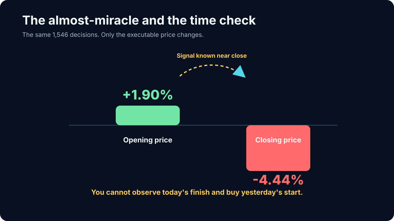

This may be the most valuable result in the series: a backtest can be arithmetically correct and operationally fictional. The profit may come not from prediction, but from combining information from one time with a price from another.

You cannot read today's information and buy yesterday's price.

Globa returned the stamp to the drawer.

AGI added a new mandatory field: signal_known_at.

Cross-bookmaker spreads: no selector, but a better receipt

The final independent odds-only branch examined opening-price disagreement across sources.

A raw difference of 0.02 means different things near 1.30 and 2.50, so we used relative price spread:

(left_odd / right_odd - 1) × 100

and implied-probability difference in percentage points.

Eight source pairs were pre-registered.

The outcome model lost to the AVG opening no-vig baseline in fixed confirmation and rolling tests. Spread states showed little persistence:

same residual sign ≈ 52.5%

That is not much more than a coin wearing a tie.

One result did survive: choosing the better available price mechanically improved execution. Across selected pairs, the average gain over the worse price was roughly:

FAV: 1.8–3.5%
DOG: 2.1–4.2%

That is not an outcome selector. It is line shopping—an execution layer.

Apparent synthetic underround still could not be called arbitrage: the opening columns lacked synchronized source timestamps, so two attractive prices may never have shared the same reality.

Again, time asked to see the documents.

What this experiment actually established

We did not prove that bookmaker odds are useless or that sports-market edge is impossible. We established a narrower result under the tested dataset, feature contracts, and time resolution:

Market Memory derivatives
H2H
consensus
opening-state buckets
movement labels
historical movement context
manual odds-only samples
cross-book disagreement

contained structure, but did not provide stable incremental outcome value over continuous market price.

Several features ranked events, reduced noise, improved description, or helped execution. None earned the title of production signal engine.

And when a positive result finally appeared, execution validation exposed a stale price.

That is what it means to make the miracle show its papers.

Do not ask only:

Is ROI positive?

Ask:

When was the signal knowable?
Which price existed then?
Did the effect survive rolling time?
Did it beat the relevant market baseline?
How many independent ideas are actually present?
What result would close the hypothesis?

After those questions, there are fewer miracles.

There is a better laboratory.